R function: plot

One (numeric) vector

plot(x) creates a scatter plot if x is a numeric vector. The values of x are plotted against their index in its vector

The following example uses type='l' to connect the points of the scatter plots with lines.

X11(width=5, height=3)

x <- 3*runif(20) + (1:20)

# png(file = 'img/vector.png', width=300, height=180)
par(mar=c(2, 2, 0.1, 0.1))
plot(x, type='l', col='#ff7733')
# dev.off()

# Wait for mouse click or enter pressed
z <- locator(1)

Github repository about-r, path: /functions/plot/vector.R

Two (numeric) vectors - scatter plot

plot(x, y) produces a scatter plot if x and y are vectors

X11(width=5, height=3)

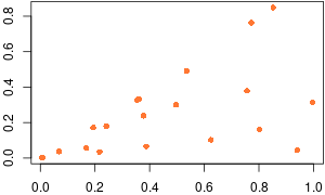
x <- runif(20)
y <- runif(20) * x

# png(file = 'img/vector-scatter_plot.png', width=300, height=180)
par(mar=c(2, 2, 0.1, 0.1))
plot(x, y, type='p', pch=16, col='#ff7733')
# dev.off()

# Wait for mouse click or enter pressed
z <- locator(1)

Github repository about-r, path: /functions/plot/vector-scatter_plot.R

Factors

If the class of the plotted variable is a factor, a bar chart is produced.

In the following example, the heights of the bars correspond to the counts of occurrences of a value in f:

X11(width=5, height=3)

f <- factor(c('foo', 'bar', 'foo', 'baz', 'bar', 'foo', 'foo', 'bar'))

# png(file = 'img/factor.png', width=300, height=180)
par(mar=c(2, 2, 0.4, 0.4))
plot(f, col='#5522cc')
# dev.off()

z <- locator(1)

Github repository about-r, path: /functions/plot/factor.R

Data frames

If a data frame is plotted, each variable of the data frame is plotted against each other.

X11(width=6, height=6)

set.seed(280870)

x <- c(4, 3, 1, 2, 2, 4, 6, 4, 5, 5, 4, 4, 5, 4, 4, 8, 4, 1, 2, 7)
y <- x * rnorm(20, 1, 0.3)
z <- x * y

df <- data.frame (x, y, z)

# png(file = 'img/data-frame.png', width=400, height=400)
par(mar=c(0.1, 0.1, 0.1, 0.1))
plot(df, col='#34b254', pch=16, cex=1.5)
# dev.off()

# Wait for mouse click or enter pressed
z <- locator(1)

Github repository about-r, path: /functions/plot/data-frame.R

Overlaying plots

A plot can be laid over another plot by setting the arg argument to TRUE:

plot(thing_one)
plot(thing_two, add = TRUE)

Plotting a subset of a data frame

The with(…) function allows to plot a specific subset of a data frame.

In the following example, only the values for item == 'baz' are plotted:

df <- read.csv(text =
"year,item,val
2014,foo,9
2014,bar,18
2014,baz,12
2015,foo,6
2015,bar,19
2015,baz,11
2016,foo,8
2016,bar,17
2016,baz,11
2017,foo,7
2017,bar,17
2017,baz,12
2018,foo,8
2018,bar,15
2018,baz,14
2019,foo,7
2019,bar,16
2019,baz,13"
);

par(mar=rep(4.2,4));

with(
   df[df$item == 'baz', ],
   plot(
     year          ,
     val           ,
     type = 'l'    ,
     lwd  =  3     ,
     col  = 'blue' ,
     xlab = 'Year' ,
     ylab = 'Value'
   )
);

Github repository about-r, path: /functions/plot/subset.R

Maximizing size of plot

In order to maximize the size of the plot itself, the margins might be set to zero (before calling plot(…)):

par(mar = c(0, 0, 0, 0))
plot(…)

TODO

x <- c(1:10)
y <- x*x - 7*x - 20

x11()

# { first example

plot(x, y, 
    main="Plot Example", # Title
    sub ="plot.R"      , # Sub title 
    xlab="x"           , # x label
    ylab="f(x)"        , # y label,
    xlim=c(-3,13)      , # range for x
    ylim=c(-40,15)     , # range for y
    col ="blue"        , # color
    pch = 19           , # 19=solid
    type="p"             # type (p = points, also possible: 
                         #       l = lines
                         #       b = both lines and points
                         #       c = b without p
                         #       o = overplotted
                         #       h = histogram
                         #       s = stair steps 
                         #       S = other steps,
                         #       n = not plotting
    )


z <- locator(1) # wait for mouse click or enter pressed

# }

# { Plot a function

plot (function(x) { x*x - 7*x - 20 },
      -2, 12)

z <- locator(1) # wait for mouse click or enter pressed

# }

# { Using different «pch» and «col» for the «dots»


d <- data.frame(
  
      foo = c(1.1, 2.0, 2.7, 2.4, 1.4, 3.3, 2.5, 1.7, 3.6, 3.3, 2.3, 3.6, 1.9, 3.8, 2.5),
      bar = c(2.9, 1.8, 2.6, 1.5, 3.3, 3.2, 1.1, 2.0, 2.9, 1.2, 2.5, 1.4, 3.1, 2.0, 1.2),
      baz = c(1  , 1  , 3  , 2  , 1  , 2  , 3  , 2  , 1  , 2  , 1  , 2  , 3  , 2  , 2  )
)

plot(d$foo, d$bar, pch=d$baz, col=c('red', 'blue', 'darkgreen')[d$baz])

z <- locator(1)

# }

Github repository about-r, path: /functions/plot.R